How to Think Clearly (6/11): Three Tools for Estimating the Unknown
Expected value, Fermi estimation and natural frequencies, plus the one estimate people reliably get wrong: their own schedule.
Where this sits: stage 4 of 6, Estimate. When the missing piece of a picture cannot be looked up, it has to be estimated, and intuition misjudges both size and odds. The safeguard is to compute. This post gives three tools for the number you do not have.
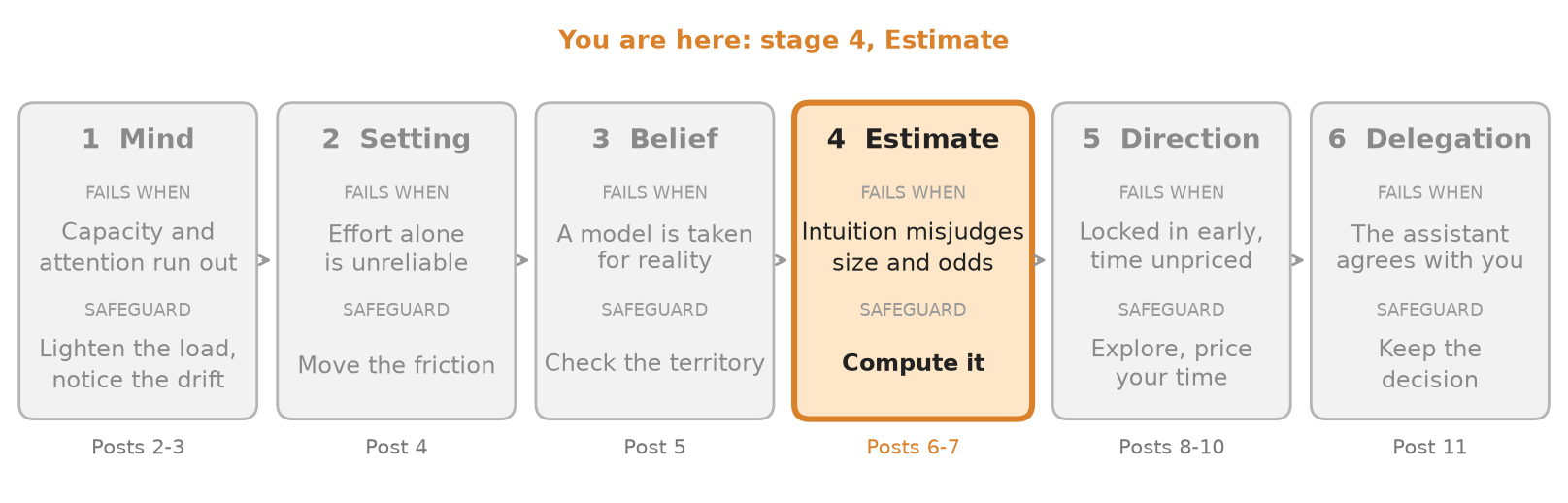 Where this post sits in the series: stage 4 of 6, Estimate.
The previous post ended with a missing piece that cannot be looked up. Most decisions are like that. This post covers three tools for working with a number you do not have: weighing outcomes, building a rough figure from parts, and updating on evidence. A fourth section covers the one estimate people reliably get wrong.
Weigh outcomes: expected value
When options have uncertain payoffs, multiply each outcome by its probability and add:
\[E[X] = \sum_i p_i x_i\]A bet that pays 100 with probability 0.3 and nothing otherwise has an expected value of 30. A sure 35 beats it on this measure. The tool is useful because it forces both numbers onto the page: the size of the prize and the chance of getting it. A large prize with a tiny probability, or a small one that is nearly certain, looks different once multiplied. (Numbers here are my own illustration.)
Its limit is that an average hides the spread. A bet repeated many times converges to its expected value; a bet you can only take once, with a loss you cannot absorb, does not. The tool answers “what is this worth on average”, not “can I survive the bad draw”.
Build a number: Fermi estimation
On 16 July 1945, at the Trinity test, Enrico Fermi dropped small pieces of paper into the blast wave and estimated the yield at 10,000 tons of TNT. The final figure was 21,000 tons, “more than twice what Fermi had estimated,” and, by the same account, four times what most people at Los Alamos had predicted. A physicist’s 2021 note points out that no account survives of how Fermi turned the paper’s motion into a yield, so the details are reconstruction. What survives is the lesson: an estimate at about half the true value, made on the spot from crude observation, was closer than most prior expert guesses.
The method generalises. Split an unknown into factors you can guess, guess each, multiply. Errors in the guesses partly cancel, because some are high and some are low. The chart below, a simulation I ran for this post, makes the point. Each of five factors is wrong by up to a factor of 3 in either direction, uniformly on a log scale. The product is usually wrong by far less than the worst case of 243:
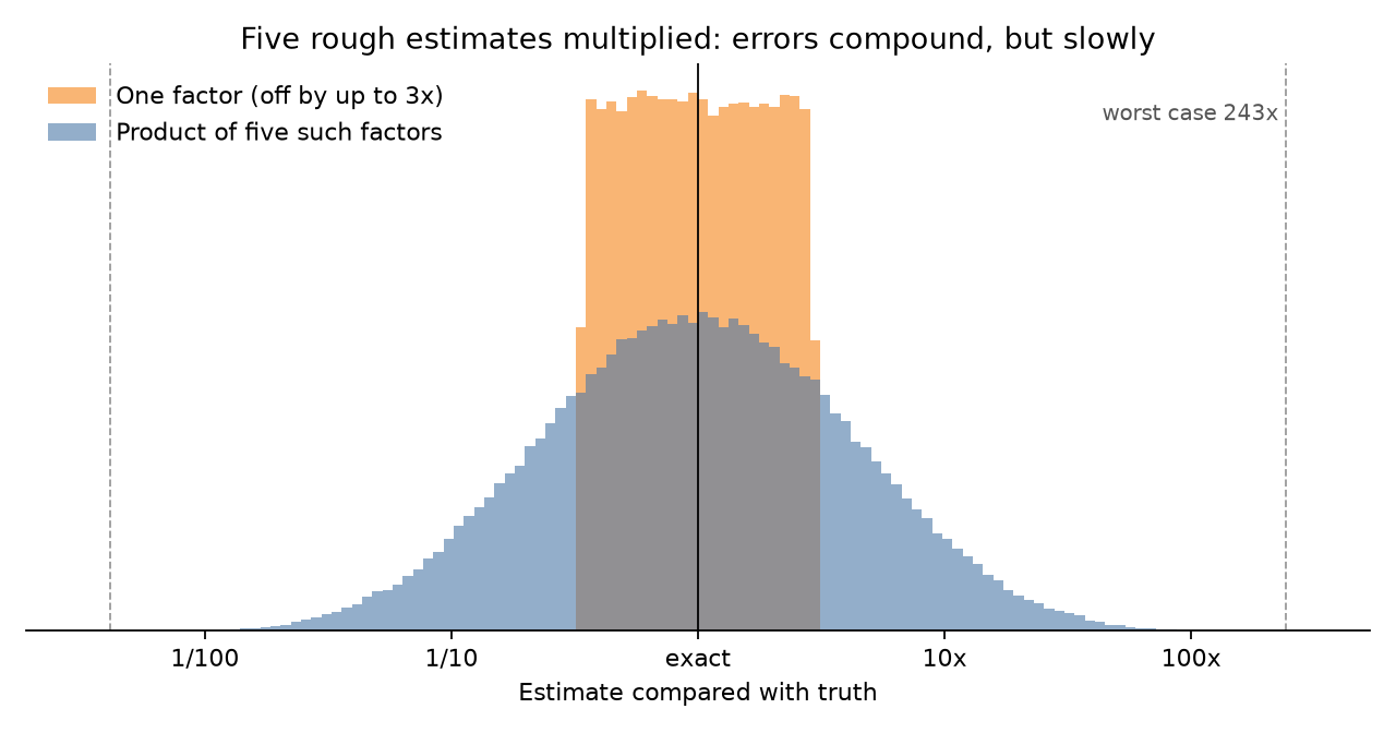 Figure 1. Simulation of 200,000 trials; the error model is an assumption of mine. In it, the five-factor product is within 2x of the truth 36% of the time, within 3x 55% and within 10x 89%.
The cancellation is a property of independent errors. If the guesses share a bias, for example all optimistic, nothing cancels, which leads to the last tool.
Update on evidence: natural frequencies
Bayes’ rule says how a prior belief should change after a test result. In probabilities it looks like this:
\[P(H\mid E) = \frac{P(E\mid H)\,P(H)}{P(E\mid H)\,P(H) + P(E\mid \lnot H)\,P(\lnot H)}\]Most people find it unintuitive. Gerd Gigerenzer and Ulrich Hoffrage showed in 1995 that the difficulty is partly the format: when the same information is given as frequencies, statistically naive participants reached Bayesian answers in up to 50% of inferences.
A standard screening example, as retold in a university course note: 1% of women aged 40 to 50 have breast cancer, a woman with cancer has a 90% chance of a positive mammogram, and a woman without has a 10% chance of a false positive. In frequencies: out of 1,000 women, 10 have cancer and 9 of them test positive; of the 990 without cancer, 99 test positive. Of 108 positives, 9 are real. The answer is 9/108, about 8%. The same note says 95 physicians asked this question averaged 75%; I could not check that survey in its original form.
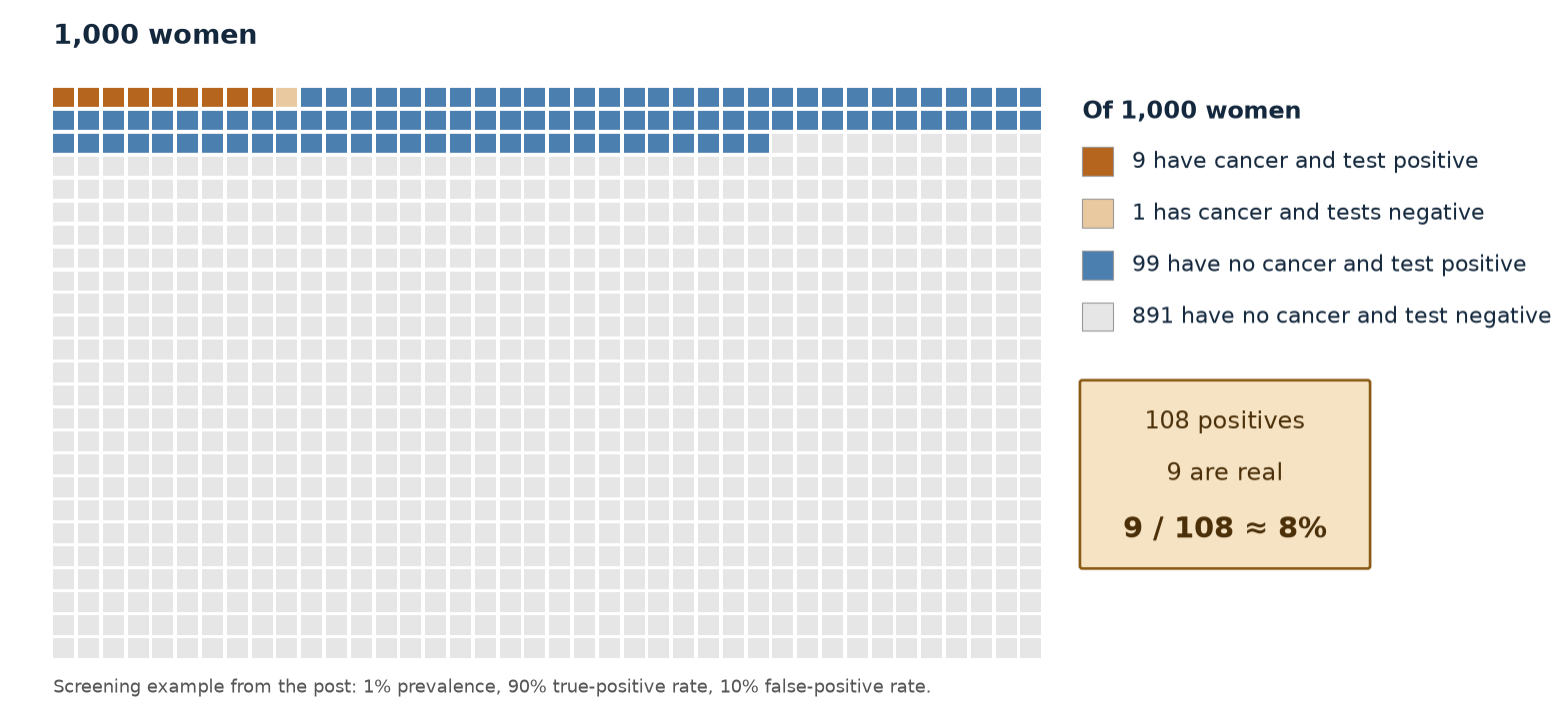 Figure 2. The screening example as counts. Of 108 positives, 9 are real, about 8%.
The counting version works for any test, not only medical ones: base rate first, then count who is flagged.
The estimate that fails: your own schedule
Fermi’s errors cancelled. Time estimates for one’s own work do not, because the bias points one way. Kahneman and Tversky named it the planning fallacy in 1979. In a 1994 study, Roger Buehler, Dale Griffin and Michael Ross asked 37 psychology students near the end of an honors thesis when they would finish. The average best-guess prediction was 33.9 days. The average actual time was 55.5 days, and 29.7% finished within the time they had predicted.
The same paper found a remedy. When participants were instructed to connect their predictions with relevant past experiences, the optimistic bias disappeared. This follows from the previous post: the prediction was built from a plan, which is a map of how things will go, and the correction is to consult the territory, meaning how similar projects actually went.
Which tool when
- The payoffs are uncertain: expected value, then ask whether the worst case is survivable.
- The number is unknown: split it, guess the parts, multiply, and check whether the guesses share a bias.
- A test or signal has arrived: write the base rate as a count and track who is flagged.
- The estimate is about your own work: replace the plan with the record of similar work.
The next post asks what shape the numbers take when they are not bell-shaped, because an average can hide the few cases that decide the outcome.
Series: How to Think Clearly. 1. Where Thinking Breaks and What to Put There. 2. A Thought Has a Machine Behind It. 3. Catch the Error While It Happens. 4. Make the Right Thing the Easy Thing. 5. The Map Is Not the Territory. 6. Three Tools for Estimating the Unknown. 7. Averages Lie. 8. Price Your Own Hour. 9. Explore Early, Exploit Late, Imagine the Failure First. 10. The Hill You Are Standing On. 11. Let AI Think, Keep the Decision.